What Is Network Throughput?
The rate at which data is processed and moved from one location to another is known as network throughput. It’s used in networking to assess the performance—or speed—of hard drives, RAM, and internet and network connections.
Bits per second or data per second are the units to measure network throughput. The network throughput of a hard disk with a maximum transfer rate of 200 Mbps is double that of a hard drive with a transfer rate of 100 Mbps. The network throughput of a 60 Mbps wireless connection is three times that of a 20 Mbps wireless connection.
The maximum network throughput of a device may be significantly higher than the actual network throughput achieved in daily use due to contributing factors such as internet connection speed and other network traffic. Generally, the realistic operational network throughput is approximately 95 percent of the maximum network throughput.
So, what is the definition of throughput? Network throughput refers to the amount of data that may be transferred from a source to a destination in a given amount of time. The number of packets that successfully arrive at their destinations is measured by throughput. Network throughput capacity is usually expressed in bits per second, although it can alternatively be expressed as data per second.
Packet arrival is critical for high-performance network service. People do use some network bandwidth analyzer pack as they expect their demands to be acknowledged and answered quickly when they utilize programs or software. Low throughput implies difficulties such as packet loss, and packet loss leads to poor or slow network performance. Maximum throughput is an effective way to assess network speed for troubleshooting since it may pinpoint the exact reason for a slow network and alert administrators to issues like packet loss.
How to Optimize Throughput
By far the most important thing to do when optimizing throughput is to minimize network latency. Latency slows down throughput which, in turn, lowers throughput and delivers poor network performance to users. Generally speaking, you want to minimize lag by monitoring endpoint usage and addressing network bottlenecks by a simple network management protocol.
The most common cause of latency is having too many people trying to use a network at the same time and reach the maximum transfer throughput capacity. Latency gets even worse if multiple people are downloading simultaneously. If you’re an IT manager, looking at endpoint usage can tell you which employees are causing latency with non-work-related applications. Even if you’re not an administrator and looking at this from a productivity bandwidth usage standpoint, it’s also helpful to know what apps are gumming up the works. Either way, information leads to action that’s why it is also important to keep measuring throughput or network performance monitor on time both throughput and bandwidth.
SNR (Signal to Noise Ratio)
The signal-to-noise ratio (SNR) is a notion that assures optimal wireless performance. The SNR is the disparity seen between received signals and the noise floor.
To correctly transfer data over an RF signal, both the transmitter and receiver must employ the same modulation algorithm. Furthermore, given the constraints, the pair should employ the highest data rate possible in their existing surroundings. A lower data rate may be preferred if they are placed in a noisy environment with a poor SNR or RSSI. If not, a greater data rate is required better.
RSSI (Received Signal Strength Indicator)
RSSI is an assumed measurement of a device’s ability to identify, identify, and pick up signals from any wireless access point or WI-FI router. An RSSI closer to 0 indicates the strength, while one closer to -100 indicates weakness.
EIRP (Equivalent Isotropic Radiated Power)
EIRP is commonly used to limit the number of radiation power emitted by wireless devices. It is defined as EIRP which is the gain of the transmitting antenna and is the input power to the transmitting antenna. It is also essential in determining transmitter power and beam verification of a 5G base station.
The reason for this is because the active antenna systems behave very differently than the isotropic antennas that have been utilized in traditional cellular applications for many years.
Increasing the output power of the transmitter is a straightforward way to overcome free space route loss.
Increased antenna gain can also increase EIRP. A higher signal intensity before free space route loss correlates to a higher RSSI value at a remote receiver following the defeat. This method may work well for a single emitter, but it might produce interference issues when many transmitters are positioned in the same region.
A more solid method would be to simply deal with the impacts of free space path loss and other negative situations. Wireless devices are often mobile and can move closer or further away from a transmitter at any time. The RSSI grows when a receiver approaches a transmitter.
This, in turn, results in a higher SNR. When the SNR is high, more sophisticated modulation and coding techniques may be utilized to convey more data. The RSSI (and SNR) falls when a receiver moves away from a transmitter. Because of the increased noise and the necessity to retransmit more data, more fundamental modulation and coding techniques are required.
DRS (Dynamic Rate Switching)
If the circumstances for high signal quality are suitable, a complicated modulation and coding system (together with a high data rate) is utilized. As the circumstances worsen, simpler methods can be chosen, resulting in a wider range but lower data rates. The scheme selection is generally referred to as dynamic rate fluctuation (DRS).
It may, as the name indicates, be conducted dynamically with no manual intervention. DRS describes a wireless station’s proclivity to negotiate at varying rates regarding the quality of the received signal from the access point.
DRS is also known by several other names, including link adaptation, adaptive modulation and coding (AMC), and rate adaptation.
Figure 1 depicts DRS operating on the 2.4 GHz band as an example. Each concentric circle reflects the range of modulation and coding schemes offered. The graph is oversimplified because it implies a constant
Across all modulation modes, power level The white circles represent OFDM modulation (802.11g), whereas the darker circles represent DSSS modulation (802.11b). To keep things simple, none of the 802.11n/ac/ax modulation modes are shown. The data rates are ordered by ascending circle size or distance from the transmitter.
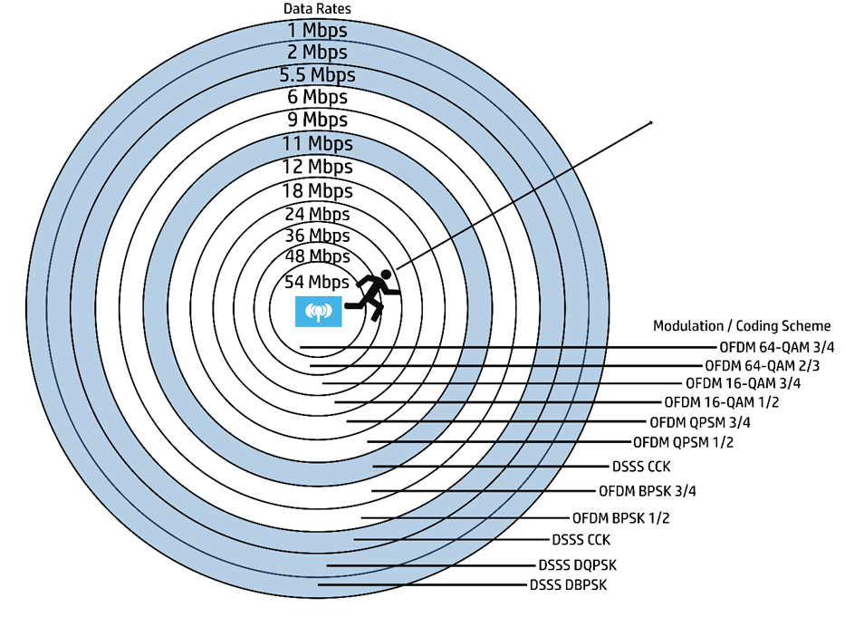
Assume a particular user begins near the transmitter, within the innermost circle, where the received signal is strong and the SNR is high. Wireless broadcasts will almost certainly utilize the OFDM 64-QAM 3/4 modulation and coding system for 54 Mbps data throughput. The RSSI and SNR decrease as the user moves away from the transmitter. The changing RF circumstances will very certainly cause a switch to a less sophisticated modulation and coding method, resulting in a decreased data rate.
In a nutshell, each step outward into a wider concentric circle results in a dynamic change to a lower data rate in an effort to preserve data integrity to the outer reaches of the network range of the transmitter, As the particular user returns to the AP, the data rates will most certainly continue to rise.
Download our Free CCNA Study Guide PDF for complete notes on all the CCNA 200-301 exam topics in one book.
We recommend the Cisco CCNA Gold Bootcamp as your main CCNA training course. It’s the highest rated Cisco course online with an average rating of 4.8 from over 30,000 public reviews and is the gold standard in CCNA training: